library(tidyverse)
library(scales)
library(viridis)
library(patchwork)

college <- read_csv('http://672258.youcanlearnit.net/college.csv') %>%
  mutate(
    state = as.factor(state),
    region = as.factor(region),
    highest_degree = as.factor(highest_degree),
    control = as.factor(control),
    gender = as.factor(gender),
    loan_default_rate = as.numeric(loan_default_rate),
    tuition_tier = cut(tuition, breaks = quantile(tuition, probs = seq(0, 1, 0.25), na.rm = TRUE), 
                      labels = c("Low", "Medium-Low", "Medium-High", "High"), include.lowest = TRUE),
    sat_category = case_when(
      sat_avg >= 1400 ~ "Elite",
      sat_avg >= 1200 ~ "High",
      sat_avg >= 1000 ~ "Medium",
      TRUE ~ "Low"
    )
  )

college_summary <- college %>%
  group_by(control, region) %>%
  summarise(
    mean_tuition = mean(tuition, na.rm = TRUE),
    mean_sat = mean(sat_avg, na.rm = TRUE),
    median_undergrads = median(undergrads, na.rm = TRUE),
    n = n(),
    .groups = 'drop'
  )

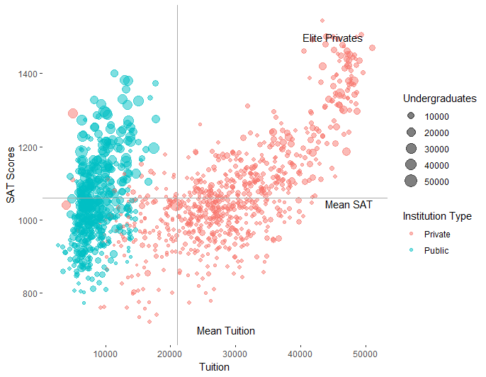
p1 <- college %>%
  filter(!is.na(tuition), !is.na(sat_avg)) %>%
  ggplot(aes(x = tuition, y = sat_avg)) +
  geom_point(aes(color = control, size = undergrads, alpha = loan_default_rate), 
             position = position_jitter(width = 200, height = 5)) +
  geom_smooth(method = "lm", se = TRUE, aes(color = control, fill = control), 
              alpha = 0.2, linetype = "dashed") +
  geom_hline(data = college_summary, aes(yintercept = mean_sat, color = control), 
             linetype = "dotted", alpha = 0.7) +
  geom_vline(data = college_summary, aes(xintercept = mean_tuition, color = control), 
             linetype = "dotted", alpha = 0.7) +
  geom_text(data = college_summary, 
            aes(x = mean_tuition, y = mean_sat, label = paste0("n=", n)),
            size = 3, hjust = -0.1, vjust = -0.5, fontface = "bold") +
  scale_color_viridis_d(name = "Institution\nType", option = "plasma", begin = 0.2, end = 0.8) +
  scale_fill_viridis_d(name = "Institution\nType", option = "plasma", begin = 0.2, end = 0.8) +
  scale_size_continuous(name = "Undergraduates", 
                       breaks = c(1000, 5000, 10000, 20000),
                       labels = c("1K", "5K", "10K", "20K"),
                       range = c(1, 8),
                       trans = "log10") +
  scale_alpha_continuous(name = "Default\nRate", range = c(0.3, 0.9)) +
  scale_x_continuous(name = "Tuition (USD)", 
                    labels = dollar_format(),
                    breaks = seq(0, 60000, 10000),
                    expand = expansion(mult = c(0.02, 0.05))) +
  scale_y_continuous(name = "Average SAT Score",
                    breaks = seq(800, 1600, 200),
                    expand = expansion(mult = c(0.02, 0.05))) +
  facet_wrap(~region, ncol = 2, scales = "free") +
  theme_minimal(base_size = 11) +
  theme(
    panel.grid.minor = element_blank(),
    panel.grid.major = element_line(color = "grey90", size = 0.3),
    panel.background = element_rect(fill = "white", color = NA),
    plot.background = element_rect(fill = "white", color = NA),
    strip.background = element_rect(fill = "grey95", color = "grey80"),
    strip.text = element_text(face = "bold", size = 11),
    legend.position = "right",
    legend.box = "vertical",
    legend.spacing = unit(0.5, "cm"),
    axis.title = element_text(face = "bold"),
    plot.margin = margin(10, 10, 10, 10)
  ) +
  guides(
    color = guide_legend(order = 1, override.aes = list(size = 4, alpha = 1)),
    size = guide_legend(order = 2),
    alpha = guide_legend(order = 3)
  )

p2 <- college %>%
  filter(!is.na(tuition), !is.na(sat_avg)) %>%
  ggplot(aes(x = tuition, y = sat_avg, fill = control)) +
  stat_density_2d(aes(alpha = ..level..), geom = "polygon", contour = TRUE, bins = 15) +
  geom_point(aes(color = control), size = 1.5, alpha = 0.6, shape = 21) +
  scale_fill_viridis_d(option = "plasma", begin = 0.2, end = 0.8, alpha = 0.6) +
  scale_color_viridis_d(option = "plasma", begin = 0.2, end = 0.8) +
  scale_x_continuous(name = "Tuition (USD)", labels = dollar_format()) +
  scale_y_continuous(name = "Average SAT Score") +
  theme_minimal() +
  theme(legend.position = "none")

p3 <- college %>%
  ggplot(aes(x = reorder(region, tuition, median, na.rm = TRUE), y = tuition, fill = control)) +
  geom_boxplot(alpha = 0.7, outlier.alpha = 0.3, width = 0.6) +
  geom_jitter(aes(color = control), width = 0.2, alpha = 0.4, size = 0.8) +
  scale_fill_viridis_d(option = "plasma", begin = 0.2, end = 0.8) +
  scale_color_viridis_d(option = "plasma", begin = 0.2, end = 0.8) +
  scale_y_continuous(name = "Tuition (USD)", labels = dollar_format()) +
  labs(x = "Region") +
  coord_flip() +
  theme_minimal() +
  theme(legend.position = "none")

final_plot <- (p1 / (p2 | p3)) + 
  plot_annotation(
    title = "Comprehensive Analysis of College Tuition vs SAT Scores",
    subtitle = "Exploring relationships across institution types and regions",
    theme = theme(plot.title = element_text(size = 16, face = "bold", hjust = 0.5),
                  plot.subtitle = element_text(size = 12, hjust = 0.5, color = "grey40"))
  )

print(final_plot)
ggsave("college_analysis.png", final_plot, width = 16, height = 12, dpi = 300, bg = "white")