How the Emax model got here
PK gives the time course of drug in plasma. PD asks what the time course of effect is. The models used routinely today were built up over about forty years, each one added because the previous one couldn’t explain something people were seeing.
Levy, 1966: effect declines linearly, concentration does not
Levy noticed that plasma concentrations fall exponentially while the measured effect of many drugs falls off in a straight line. Writing $E$ for effect:
\[E = E_0 - k \cdot m \cdot t\]where $k$ is the elimination rate constant and $m$ is the slope of the effect against log concentration. This works because effect is roughly linear in log concentration over the middle of its range, and log concentration falls linearly with time, so $k \cdot m$ sets how fast effect decays.
It only holds over that middle range, roughly 20% to 80% of maximum effect. Outside it the relationship breaks down, because effect saturates and concentration doesn’t.
Wagner, 1968: borrowing the Hill equation
Wagner described the saturation directly, using the equation A.V. Hill had derived in 1910 for oxygen binding to haemoglobin, which follows from the same mass-action reasoning as drug binding to a receptor:
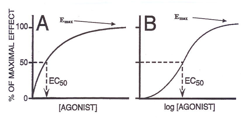
\[E(t) = \frac{E_{max} \cdot C(t)^{\gamma}}{EC_{50}^{\gamma} + C(t)^{\gamma}}\]$E_{max}$ is the maximum achievable effect, $EC_{50}$ the concentration giving half of it, and $\gamma$ the Hill coefficient controlling how steeply effect turns on. This is the Emax model. Because saturation is built in, it holds across the whole concentration range and the 20-80% restriction goes away.
Segre and Sheiner: effect lags concentration
As written, the Emax model assumes peak effect happens at peak concentration. For most drugs it doesn’t. Effect lags, and a plot of effect against concentration traces a loop instead of a curve (hysteresis).
Segre’s idea, which Sheiner and colleagues made standard in 1979 with d-tubocurarine, was to add a hypothetical effect compartment: a small, kinetically separate space that the drug equilibrates into with its own rate constant. Effect is still given by the Emax equation, but driven by the concentration in that compartment instead of plasma. The delay is then a distribution delay, and by construction it doesn’t change the plasma PK.
Ariëns, Nagashima, Jusko: when the delay is not distribution
An effect compartment explains delays of minutes to hours. It can’t explain delays of days, or a response that keeps changing after the drug is gone.
Those delays happen when the drug acts on the turnover of the measured quantity rather than on the quantity itself. Ariëns argued for indirect mechanisms as early as 1954, and Nagashima and colleagues built the first quantitative example in 1969 for warfarin, which doesn’t change clotting time directly but suppresses synthesis of the clotting factors that determine it. Dayneka and Jusko later organised these into four basic models, depending on whether the drug inhibits or stimulates production ($k_{in}$) or loss ($k_{out}$):
\[\frac{dR}{dt} = k_{in} \cdot H_1(C) - k_{out} \cdot H_2(C) \cdot R\]where $H_1$ and $H_2$ are Emax-type functions of concentration and $R_0$ is the baseline. The time course of the response is now set by the turnover of the biomarker rather than the PK, which is why washout after stopping the drug can take much longer than the drug’s own half-life.
One way to tell the two apart: in an effect-compartment model the time to peak effect doesn’t depend on dose, while in an indirect response model it moves later as dose goes up, because concentrations stay above $EC_{50}$ for longer.
Transit compartments
Some systems show no change at all for a while after dosing, even at high concentrations (signal transduction cascades, for example). The usual approach is a chain of transit compartments, which adds an adjustable delay with few extra parameters.
Most PK/PD models since then build on these four ideas: saturation, distribution delay, turnover and transduction delay.
Reading an Emax curve
The curve is a good way to keep potency and efficacy apart, since they get mixed up a lot:
- Potency is $EC_{50}$, read off the x-axis: how much drug you need.
- Efficacy is $E_{max}$, read off the y-axis: how much effect you can get at all.
They’re independent and neither predicts the other. A very potent drug with low efficacy reaches its modest ceiling at a low dose. A low-potency drug with high efficacy needs a lot of drug but can push the response further. So comparing two drugs on $EC_{50}$ alone tells you about dose size and nothing about what the drug can achieve.
References
- Hill AV. The possible effects of the aggregation of the molecules of haemoglobin on its dissociation curves. J Physiol. 1910;40:iv-vii.
- Ariëns EJ. Affinity and intrinsic activity in the theory of competitive inhibition. Arch Int Pharmacodyn Ther. 1954;99(1):32-49.
- Levy G. Kinetics of pharmacologic effects. Clin Pharmacol Ther. 1966;7(3):362-372.
- Wagner JG. Kinetics of pharmacologic response I. J Theor Biol. 1968;20(2):173-201.
- Nagashima R, O’Reilly RA, Levy G. Kinetics of pharmacologic effects in man: the anticoagulant action of warfarin. Clin Pharmacol Ther. 1969;10(1):22-35.
- Sheiner LB, Stanski DR, Vozeh S, Miller RD, Ham J. Simultaneous modeling of pharmacokinetics and pharmacodynamics: application to d-tubocurarine. Clin Pharmacol Ther. 1979;25(3):358-371.
- Dayneka NL, Garg V, Jusko WJ. Comparison of four basic models of indirect pharmacodynamic responses. J Pharmacokinet Biopharm. 1993;21(4):457-478.
- Jusko WJ, Ko HC. Physiologic indirect response models characterize diverse types of pharmacodynamic effects. Clin Pharmacol Ther. 1994;56(4):406-419.
- Mager DE, Jusko WJ. Pharmacodynamic modeling of time-dependent transduction systems. Clin Pharmacol Ther. 2001;70(3):210-216.